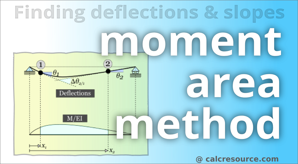
This is a method for the calculation of deflections of beam structures that rely on the shape of bending moment diagram. It was improvised by Christian Otto Mohr (1835-1918). Usually, no integration is needed, so it proves more convenient in terms of calculation efficiency and therefore can be effective to more complex structural geometries, compared to direct integration method. It is better suited to cases where the areas and centroids of the regions in the bending moment diagram are easy to determine. For example when there only point loads imposed on the structure. In that case the bending moment diagram consist of triangular or rectangular regions.
Classical beam theory
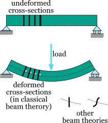
Trying to estimate the deformations of a beam under transverse loading several beam theories are available. The most widely adopted is the Euler-Bernoulli beam theory, also called classical beam theory. The two basic assumptions of the theory are:
the deformations remain small
the cross sections of the beam under deformation, remain normal to the deflected axis (aka elastic curve).
The second assumption is practically valid for beams with homogeneous and isotropic material, with symmetrical cross-section, and with length significantly larger than their cross section dimensions (10 times or more is a common rule of thumb). Effectively, if the the beam deforms significantly in any other form except symmetric bending then the assumption of normal and plane cross sections is not satisfied. Examples of such cases include short beams, beams with sandwich type cross-sections, or slender cross-sections or open unsymmetrical cross-sections.
Also the following assumptions are typically associated with the classical beam theory:
the material is linear elastic
the beam is prismatic, which means that the cross-section remains constant throughout its length
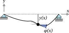
Under these assumptions, the classical beam theory results to the following relationship between the deflection , as a function of and the bending moment :
where, is the modulus of elasticity and the moment of inertia of the cross section.
Moment area theorems
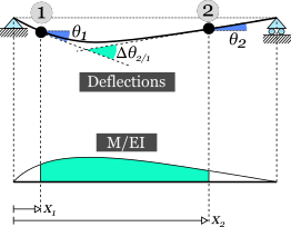
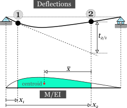
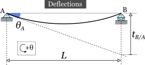
The moment area method is based on two theorems, also called 'moment area theorems' or 'Mohr's theorems'. The first one correlates the slope change between any two points of the beam, while the second one is related with the deflection at a point of the beam. The two theorems will be presented after the following schematic, that will be used as a reference. It illustrates a simple beam, deflected by some random loading, and the corresponding bending moment diagram.
Theorem 1
The change of slope between any two points of the elastic curve is equal to the area of the bending moment diagram, between these two points, divided by .
Slopes are measured in radians for the needs of the moment area method.
The following schematic, illustrates a simple beam, deflected by some random loading. The change of slope , between points 1 and 2 is highlighted as well as the area of the diagram between these two points. If is constant throughout the beam, the first moment area theorem can be formulated in the following expression:
where , the x coordinates of points 1 and 2. The integral is the area of the bending moment diagram between points 1 and 2. In many cases, the area can be found analytically, avoiding integration completely.
Theorem 2
The deviation of the elastic curve at any point, from the slope line, projected from another point, is equal to the first moment of area, about the first point, of the bending moment diagram, between the two points, divided by .
The following figure depicts the deflected geometry of a simply supported beam and the respective diagram. Also it highlights the deviation of the elastic curve at point 2 from the slope line projected from point 1, as well as the centroid of the area enclosed by the diagram between the two points 1 and 2. Assuming is constant throughout the beam span, the second moment area theorem can be formulated with:
The integral term is equal to the first moment of area of the diagram about point 2 (also called static moment). In many cases it can be simplified to analytical evaluation. For example, if the centroid of the area is available, the above expression becomes:
The above integral represents the area of the diagram, between points 1 and 2, similar to the first theorem. It may be possible to evaluate it analytically, skipping integration completely.
Note that the centroid of the diagram is measured from the point where the deviation is evaluated (e.g. point 2 in the schematic). In general:
Sign convention
The following rules should be used for the interpretation of signs of the slope change and deflection deviation , in the context of the moment area method, though in many cases intuition alone is adequate.
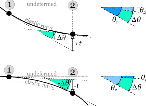
When the change in slope between two points of the elastic curve is positive, then a counter-clockwise rotation should be applied to the slope of the first point, in order to get the slope at the second point. On a negative slope change, a clockwise rotation should be applied instead.
When the deflection deviation is positive, then the elastic curve, at the examined point, lies towards the undeformed position of the same point (i.e. to get the deflected point we have to move upwards from the projected slope line).
The following figure depicts two examples for both positive (top) and negative (bottom) slope change and deviation.
It is important to note that the above convention for the slope change is independent from the sign convention used for the measurement of slopes themselves. If the slopes are measured in a counter-clockwise direction (as they typically do), then slopes and in the last figure are both negative (the rotation from the unreformed line is clockwise). Therefore, the appropriate algebraic expression for the relationship between, and the respective individual slopes should be:
On the other hand, if the slopes are measured in a clockwise direction then both and are positive. So the appropriate algebraic expression this time should be:
Of course, it is more intuitive to use the same convention for both slope measurement and slope change measurement.
Always pay attention to the geometry of the problem and assign the appropriate sign to the calculated slopes and deflections.
Using the Moment Area Theorems
The moment area theorems rely on the bending moment diagram, so at first this should have been determined. Secondly, drawing a rough sketch of the expected deflected shape of the structure proves quite helpful, because the methodology uses the the geometric relationships between slopes and deflections, that are specific to the examined structure. Depending on the supports, some points of the elastic curve should have fixed deflections or slopes. Beginning with these points, we can find the deflections and slopes at any other point. Some practical rules can be helpful in this context:
If the the deflection is known at any two points of a continuous beam, then we can use the second moment area theorem to find the slope at either one of the two points.
If the slope is known to any point of a continuous beam, then we can use the first moment area theorem to find the slope at any other point of the beam.
If both the deflection and the slope is known at any point of a continuous beam, then we can use the second moment area theorem to find the deflection at any other point of the beam
If the beam is discontinuous at some point (i.e. there is an internal hinge), then the moment area method can still be used, but separately on each side of the discontinuity. A sketch of the deflected shape is very helpful in this case.
In the case of simply supported beam there are two supports, a pin and a roller, both of which enforce zero deflection of the beam. Therefore, at these two points deflection is known and equal to 0. We can use the rules 1 and 3 to solve most problems, requiring evaluation of deflections. Rules 1 and 2 are suitable when a slope is required.
In the case of a cantilever beam, there is only one support. Because it is a fixed support, both deflection and slope of the beam should be zero at this point. As a result, we may use rule 3 alone, to find the deflection, at any other point, and rule 2 alone to find the slope.
Example 1: deflections of a simply supported beam with point load, using the moment area method
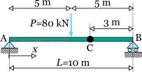
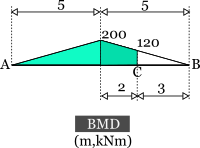
Find the deflection and slope at point C of the simply supported beam, shown in the figure, having an imposed point force at the middle. It is , constant over the entire beam span.
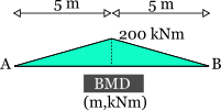
Before we begin, we have to determine the bending moment diagram. Since there is no distributed load the diagram should be linear. The maximum occurs at the middle point and it turns out to be:
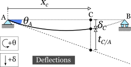
1. Finding the deflection and slope at point C
A sketch of the deflected shape is first drawn. It is known that at the two supports the deflection is zero. Therefore, the deviation of the elastic curve, say at the end point B, measured from the slope at A, should be equal to:
However, the deviation can be determined from the second moment area theorem. The procedure requires to find the static moment of the bending moment diagram between points A and B (the whole diagram) about point B. The centroid of the diagram lies in the middle, therefore its distance from point B is:
The area of the diagram is also found:
Applying the second theorem we get:
Therefore:
But assuming a counter-clockwise direction for slopes, the slope at A should be negative! We have introduced a sign error with our initial geometric assumption . Taking into account the sign convention for slopes we should have used instead: . However, the examined case is quite simple, and intuition can solve such issues. We assign the appropriate sign to :
Now that the slope at A is known, we can find the deflection and slope at point C. For the slope , the first theorem is applicable. The procedure requires the calculation of the BMD area between A and C. It is more convenient to divide the BMD area into two parts: a triangular and a trapezoidal one, as shown in the figure:
It is:
Applying the first moment area theorem we get:
The slope change is positive, therefore the slope from A must rotate counter-clockwise in order to match slope at C (as expected). The slopes are also measured counter-clockwise, so the change slope in algebraic terms is defined as:
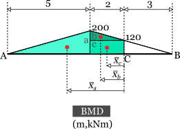
To find the deflection at C too, we can use the second theorem. This requires the static moment of the BMD area, between points A and C, about point C. For this calculation, it is convenient to divide the BMD area into three parts, a,b and c, as shown in the following figure.
The static moment for each part is the product of its area times the distance of its centroid, measured from C. Thus, we calculate the area and the centroid for each part.
Areas:
Centroids:
Static moments:
In a tabular form:
Part
Area (kNm2)
Centroid (m)
Static moment (kNm3)
a
500
3.667
1833,3
b
80
1.333
106,7
c
240
1
240
The static moment of the complete BMD area is the sum of the static moments of the parts:
Applying the second moment area theorem we find the deviation of the elastic curve:
Inspecting, the geometry, the relation between deviation and the wanted deflection at C is defined:
Example 2: deflections of a cantilever beam using the moment-area method
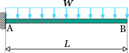
Determine the deflection and the slope at the tip of a cantilever beam, loaded by a uniform distributed load over its entire span. is constant.
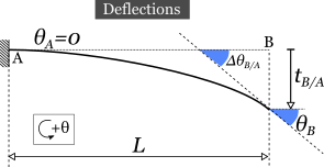
The bending moment diagram of a cantilever beam with a uniform distributed load is given in the following figure. The curve is parabolic, with zero slope at point B.
The fixed support of the cantilever beam enforces zero deflection and slope at point A.
A sketch of a the deflected is first drawn. Since the slope at A is zero, the projected slope line from A coincides with the undeformed line of the beam. As a result, the deviation of the deflected shape at point B, from the slope line, projected from A, is identical to the deflection itself .
Also, the slope change from A to B, is equal to the slope at B itself.
[\Delta\theta_{B/A}=\theta_B\]
Finding deflection at tip B
Since , we can use the second moment area theorem to find the deviation , and also deflection .
According to 2nd theorem, we have to find the static moment of the bending moment diagram between points A and B (the whole diagram) about point B. To this end, the area of the diagram and its centroid (measured from B) will be calculated. Taking reference from the table, later in the text, the following formulas are used:
Therefore, the static moment is:
Applying the second moment area theorem we get:
Thus the downward deflection at B is:
Finding slope at tip B
Since , we can use the first moment area theorem to find the slope change , and also slope .
According to 1st theorem, we have to find the area of the bending moment diagram between points A and B (the whole diagram). It has already been determined:
Applying the first moment area theorem we get:
Thus the slope at B is:
The negative sign indicates a clockwise rotation.
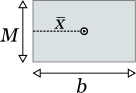
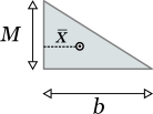
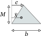
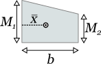
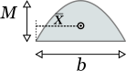
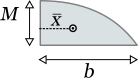
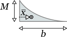
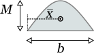
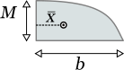
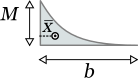
Areas and centroids of common shapes
The following table presents the formulas for the area and the centroid of several shapes, commonly encountered in bending moment diagrams.