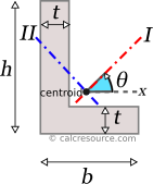
Angle (L) Section Calculator
This tool calculates the properties of an angle cross-section (also called L section). Enter the shape dimensions h, b and t below. The calculated results will have the same units as your input. Please use consistent units for any input.
h = | |||
b = | |||
t = | |||
Geometric properties: | |||
Area = | |||
Perimeter = | |||
xc = | |||
yc = | |||
Properties related to x-x axis: | |||
Ix = | |||
Sx = | |||
Zx = | |||
ypna = | |||
Rgx = | |||
ADVERTISEMENT | |||
Properties related to y-y axis: | |||
Iy = | |||
Ixy = | |||
Sy = | |||
Zy = | |||
xpna = | |||
Rgy = | |||
Properties related to major principal axis I: | |||
II = | |||
θI (°) = | |||
SI = | |||
RgI = | |||
Properties related to minor principal axis II: | |||
III = | |||
θII (°) = | |||
SII = | |||
RgII = | |||
Other properties: | |||
Iz = | |||
 |
ADVERTISEMENT
Definitions
Table of contents
Geometry
The area A and the perimeter P of an angle cross-section, can be found with the next formulas:
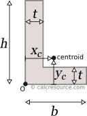
The distance of the centroid from the left edge of the section , and from the bottom edge , can be found using the first moments of area, of the two legs:
We have a special article, about the centroid of compound areas, and how to calculate it. Should you need more details, you can find it here.
Moment of Inertia
The moment of inertia of an angle cross section can be found if the total area is divided into three, smaller ones, A, B, C, as shown in the figure below. The final area, may be considered as the additive combination of A+B+C. However, a more straightforward calculation can be achieved by the combination (A+C)+(B+C)-C. Also, the calculation is better done around the non-centroidal x0,y0 axes, followed by application of the the Parallel Axes Theorem.
First, the moments of inertia Ix0, Iy0 and Ix0y0 of the angle section, around the x0, and y0 axes, are found like this:
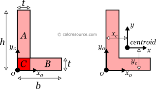
Application of the Parallel Axes Theorem makes possible to find the moments of inertia around the centroidal axes x,y:
where, the distance of the centroid from the y0 axis and the distance of the centroid from x0 axis. Expressions for these distances are given in the previous section.
Take in mind, that x, y axes are not the natural ones, the L-section would prefer to bend around, if left unrestrained. These would be the principal axes, that are inclined in respect to the geometric x, y axes, as described in the next section.
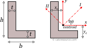
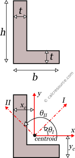
Principal axes
Principal axes are those, for which the product of inertia Ixy, of the cross-section becomes zero. Typically, the principal axes are symbolized with I and II and are perpendicular, one with the other. The moments of inertia, when defined around the principal axes, are called principal moments of inertia and are the maximum and minimum ones. Specifically, the moment of inertia, around principal axis I, is the maximum one, while the moment of inertia around principal axis II, is the minimum one, compared to any other axis of the cross-section. For symmetric cross-sections, the principal axes match the axes of symmetry. However, there is no axis of symmetry in an L section (unless for the special case of an angle with equal legs), and as a result the principal axes are not apparent, by inspection alone. They must be calculated, and in particular, their inclination, relative to some convenient geometric axis (e.g. x, y), should be determined.
Knowing the moments of inertia , and the product of inertia , of the L-section, around centroidal x, y axes, it is possible to find the principal moments of inertia , around principal axes I and II, respectively, and the inclination angle , of the principal axes from the x, y ones, with the following formulas:
By definition, is considered the major principal moment (maximum one) and the minor principal moment (minimum one). It follows that: .
Moment of inertia and bending
The moment of inertia (second moment or area) is used in beam theory to describe the rigidity of a beam against flexure. The bending moment M applied to a cross-section is related with its moment of inertia with the following equation:
where E is the Young's modulus, a property of the material, and the curvature of the beam due to the applied load. Therefore, it can be seen from the former equation, that when a certain bending moment M is applied to a beam cross-section, the developed curvature is reversely proportional to the moment of inertia I.
Polar moment of inertia of L-section
The polar moment of inertia, describes the rigidity of a cross-section against torsional moment, likewise the planar moments of inertia described above, are related to flexural bending. The calculation of the polar moment of inertia around an axis z-z (perpendicular to the section), can be done with the Perpendicular Axes Theorem:
where the , , the moments of inertia around axes x-x and y-y, respectively, which are mutually perpendicular to z-z and meet at a common origin.
The dimensions of moment of inertia are .
Elastic section modulus
The elastic section modulus of any cross section around centroidal axis x-x, describes the response of the section under elastic flexural bending. It is defined as:
where , the moment of inertia of the section around x-x axis and , the distance from centroid of a given section fiber (that is parallel to the axis). For the angle section, due to its unsymmetry, the is different for a top fiber (at the tip of the vertical leg) or a bottom fiber (at the base of the horizontal leg). Normally, the more distant fiber (from centroid) is considered when finding the elastic modulus. This happens to be at the tip of the vertical leg (for bending around x-x). Using the possibly bigger , we get the smaller , which results in higher stress calculations, as will be shown shortly after. This is usually preferable for the design of the section. Therefore:
where the “min” or “max” designations are based on the assumption that , which is valid for any angle section.
Similarly, for the elastic section modulus , relative to the y-y axis, the minimum elastic section modulus is found with:
where the “min” designation is based on the assumptions that , which again is valid, for any angle section.
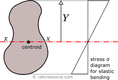
If a bending moment is applied on axis x-x, the section will respond with normal stresses, varying linearly with the distance from the neutral axis (which under elastic regime coincides to the centroidal x-x axis). Over the neutral axis the stresses are by definition zero. Absolute maximum stress will occur at the most distant fiber, with magnitude given by the formula:
From the last equation, the section modulus can be considered for flexural bending, a property analogous to cross-sectional A, for axial loading. For the latter, the normal stress is F/A.
The dimensions of section modulus are .
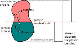
Plastic section modulus
The plastic section modulus is similar to the elastic one, but defined with the assumption of full plastic yielding of the cross section, due to flexural bending. In that case, the whole section is divided in two parts, one in tension and one in compression, each under uniform stress field. For materials with equal tensile and compressive yield stresses, this leads to the division of the section into two equal areas, , in tension and , in compression, separated by the neutral axis. This axis is called plastic neutral axis, and for non-symmetric sections, is not the same with the elastic neutral axis (which again is the centroidal one). The plastic section modulus is given by the general formula:
where the distance of the centroid of the compressive area from the plastic neutral axis and the respective distance of the centroid of the tensile area .
Around x axis
For the case of an angle cross-section, the plastic neutral axis for x-x bending, can be found by either one of the following two equations:
which becomes:
where , the distance of the plastic neutral axis from the bottom end of the section. The first equation is valid when the plastic neutral axis passes through the vertical leg, while the second one when it passes through the horizontal leg. Generally, it can't be known which equation is relevant beforehand.
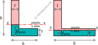
Once the plastic neutral axis is determined, the calculation of the centroids of the compressive and tensile areas becomes straightforward. For the first case, that is when the axis crosses the vertical leg, the plastic modulus can be found like this:
which becomes:
where .
For the second case, that is when the axis passes through the horizontal leg, the plastic modulus is found with equation:
which can be simplified to:
where .
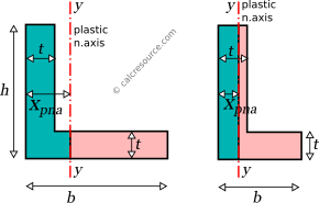
Around y axis
The plastic section modulus around y axis can be found in a similar way. If we orient the L-section, so that the vertical leg becomes horizontal, then the resulting shape is similar in form with the originally oriented one. Thus, the derived equations should have the same form, as found for the x-axis. We only have to swap for and vice-versa. This way, the exact position of the plastic neutral axis is given by the following formula:
where , the distance of the plastic neutral axis from the left end of the section. The first equation is valid when the plastic neutral axis passes through the horizontal leg, while the second one when it passes through the vertical leg (see figure below).
For the first case, that is when the y-axis crosses the horizontal leg, the plastic modulus is found by the formula:
where .
For the second case, that is when the y-axis crosses the vertical leg, the plastic modulus is found by the formula:
where .
Radius of gyration
Radius of gyration Rg of a cross-section, relative to an axis, is given by the formula:
where I the moment of inertia of the cross-section around the same axis and A its area. The dimensions of radius of gyration are . It describes how far from centroid the area is distributed. Small radius indicates a more compact cross-section. Circle is the shape with minimum radius of gyration, compared to any other section with the same area A.
Angle (L) section formulas
The following table, lists the main formulas for the mechanical properties of the angle (L) cross section.